Rational Decisions & Classical ML
Data → prediction → utility → action. A model that predicts well is not automatically a system that decides well.
Part 1: Choosing under uncertainty
Recall: a rational agent maximises expected performance using the evidence available before acting. A bad outcome doesn't prove a bad decision. Probability alone isn't enough either: 90% success can be unattractive if failure is catastrophic. We need a utility, a number for how much we prefer each outcome.
| Success | Failure | Expected utility | |
|---|---|---|---|
| Project A | 90% · (+100) | 10% · (−20) | 90 − 2 = 88 |
| Project B | 60% · (+200) | 40% · (−50) | 120 − 20 = 100 ★ |
B has a lower success probability but a higher expected utility, so a risk-neutral agent picks B. A risk-averse agent (concave utility for money) might still prefer A. Utility encodes preferences; it isn't the same as money.
From belief to action: the maintenance threshold
Bayesian inference tells us what to believe; decision theory tells us what to do. If continuing costs p·C_failure in expectation and maintenance costs C_maint (and fully prevents failure):
The threshold of 20% follows from costs, not from model accuracy. Practice: p = 15%, failure = $20,000, maintenance = $2,000. Continuing costs 0.15·20,000 = $3,000 in expectation, more than $2,000, so maintain and save $1,000 in expectation.
The spam decision (lecture example)
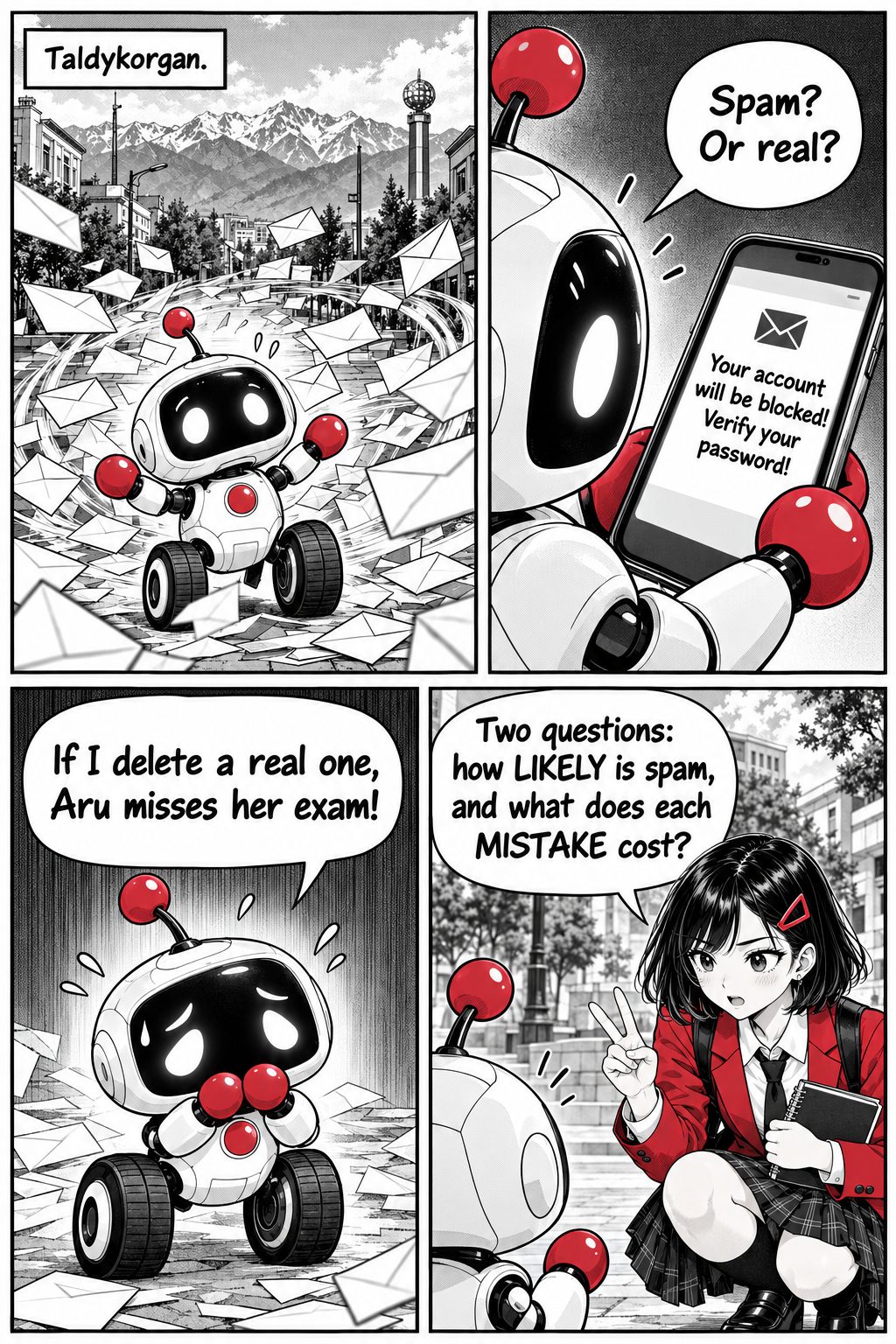
Suppose P(Spam) = 0.8. Deleting a legitimate message costs 100, delivering spam costs 5, and a quarantine folder costs 2 either way.
| Action | Expected cost | EU |
|---|---|---|
| Delete | 0.8·0 + 0.2·100 = 20 | −20 |
| Deliver | 0.8·5 + 0.2·0 = 4 | −4 |
| Quarantine | 0.8·2 + 0.2·2 = 2 | −2 ★ |
An "80% spam" prediction still shouldn't be deleted! Deleting beats delivering only when P(Spam)·5 > (1 − P)·100, which means P(Spam) > 100/105 ≈ 95.2%.
Part 2: Machine learning
Classical programming: humans write the rules (IF temperature > 80: alarm). Real data are noisy, classes overlap and patterns are nonlinear. Machine learning takes examples with outcomes and learns a model ŷ = fθ(x) with parameters θ that predicts new cases.
Workflow: collect labelled examples → split into training and test sets → fit → evaluate on unseen data → deploy. Avoid data leakage: test information must never influence training.
Supervised
Learn from labelled examples (input → known answer). Failure detection, spam filtering. Algorithms: regression, trees, Naive Bayes.Unsupervised
Find structure without labels. Customer segments, operating modes. Algorithms: K-Means, PCA.Reinforcement
Learn a policy from rewards by trial and feedback (Chapter 5). Robot control, maintenance timing.Regression: predict a number
Training finds w and b that minimise the mean squared error (MSE). Other metrics: MAE, RMSE, R².
Classification: predict a class or a probability
Logistic regression squeezes a linear score into a probability with the sigmoid:
A class decision still needs a threshold τ. The default 0.5 is not always right: when missed failures are expensive, τ might be 0.2 or lower. The threshold is a decision policy, not a property of the model.
Decision trees learn transparent IF–THEN splits ("Temperature > 70 °C? → Vibration > 3? → Failure"). They're easy to explain but deep trees overfit. Random forests train many trees on bootstrap samples with random feature subsets and vote, which lowers variance. k-nearest neighbours classifies a point by the majority label of its k closest training examples.
Naive Bayes: Bayes' theorem + a bold assumption
Assume the words are conditionally independent given the class (the "naive" part). Then:
The assumption is usually false (words come in phrases), yet Naive Bayes works well for text, trains in one pass and was the classic spam filter for years.
Trained on 12 tiny example messages (6 spam, 6 legitimate) with Laplace smoothing (+1 to every word count, so a known word missing from one class doesn't zero everything out). Words never seen in training are ignored.
P(Spam | message) = – → decision: –
Evaluating classifiers: accuracy is not enough
The 98% trap: if only 2% of machines fail, a model that always says "normal" is 98% accurate with 0% recall. Model A (95% accuracy, 60% recall) can be worse than Model B (92% accuracy, 90% recall) when missed failures are dangerous.
20 machines sorted by the model's failure score (0 → 1). Red = actually failed, white = fine.
Unsupervised: K-Means clustering
No labels, only similarity. K-Means: choose K centroids → assign each point to the nearest → move each centroid to the mean of its points → repeat until stable. It minimises J = Σₖ Σx∈Cₖ ‖x − μₖ‖². Scale features first (spending in tenge would swamp purchase counts), and remember that cluster numbers have no meaning until a human interprets them.
Risks that break real systems
- Overfitting: memorising noise. Great on training data, poor on new data.
- Data leakage: using information that won't be available at prediction time.
- Distribution shift: new conditions differ from the training data (a new machine model, winter instead of summer).
- Calibration error: "70% risk" should come true about 70% of the time. For decisions, trustworthy probabilities can matter more than raw accuracy.
Banks flag fraud with classifiers and then choose actions by cost: block the card, send an SMS check, or allow. Factories predict failure and maintain by threshold. Hospitals tune recall high for screening tests. The ML model provides the probability; the cost model provides the decision.
People struggle to combine many weak clues consistently; simple statistical models often beat expert intuition at that. Humans are far better at noticing when the situation is new and the model's assumptions no longer hold. Good systems keep both in the loop.
1. Route A: 80% success (+100) / 20% failure (−50). Route B: 95% (+80) / 5% (−20). MEU chooses…
2. Only 2% of cases are failures. A model always predicting "normal" has accuracy…
3. Maintenance costs $2,000, failure costs $10,000. Maintain when P(failure) exceeds…
4. Grouping customers with no labels is…