Probability & Bayesian Networks
Evidence is not proof. Probability is how a rational agent measures how much to believe.
Why AI needs probability
Real observations are incomplete, noisy and sometimes contradictory. A fever doesn't prove a particular disease; a hot motor doesn't guarantee failure. A rational agent assigns degrees of belief to competing explanations and updates them as evidence arrives.
The basics
- A random variable maps uncertain outcomes to values: Rain ∈ {true, false}; Weather ∈ {sunny, cloudy, rainy}.
- A distribution gives every outcome a probability, and they sum to 1: 0.50 + 0.30 + 0.20 = 1.
- Joint probability P(A, B): both happen. Conditional probability P(A | B): A happens, given that we know B.
Conditioning = shrinking the world
| 100 days | Heavy traffic | Light traffic | Total |
|---|---|---|---|
| Rain | 24 | 6 | 30 |
| No rain | 21 | 49 | 70 |
| Total | 45 | 55 | 100 |
P(Heavy) = 45/100 = 45%. But P(Heavy | Rain) = 24/30 = 80%. Conditioning changed the denominator from all 100 days to only the 30 rainy days.
Bayes' theorem
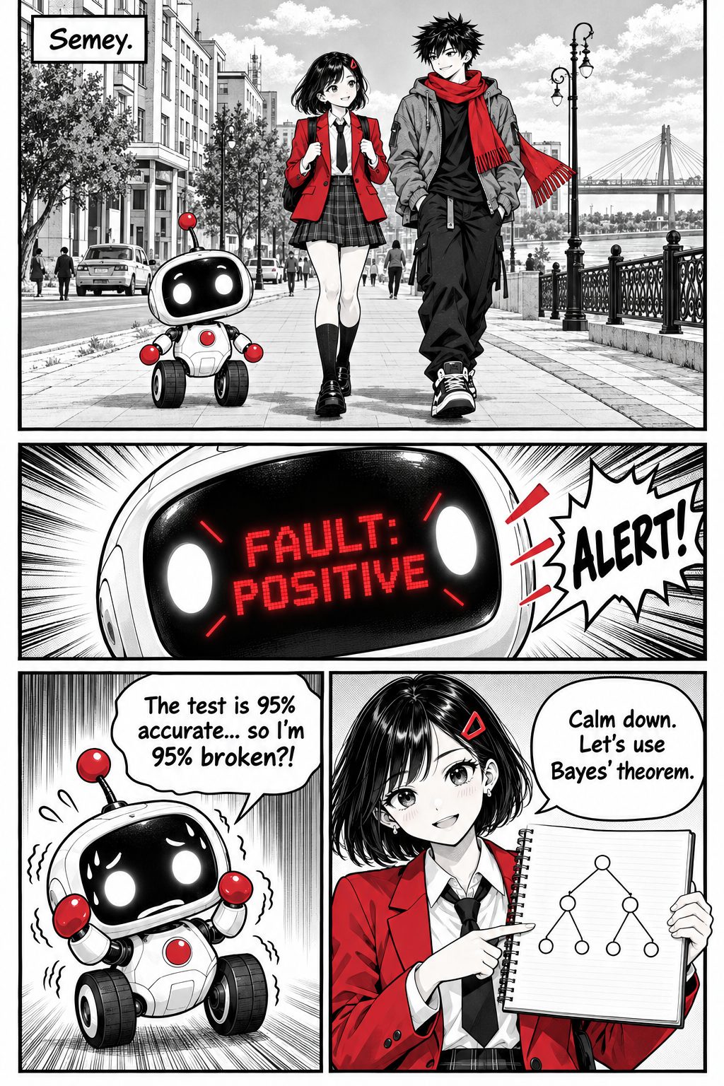
Bota's test: prevalence (prior) P(Fault) = 1%, sensitivity P(+ | Fault) = 95%, false-positive rate P(+ | ¬Fault) = 10%.
- P(+) = 0.95·0.01 + 0.10·0.99 = 0.0095 + 0.099 = 0.1085
- P(Fault | +) = 0.0095 / 0.1085 = 0.0876 ≈ 8.76%
In natural frequencies: of 10,000 robots, 100 are faulty, and 95 of them test positive. Of the 9,900 healthy ones, 990 also test positive. Among 1,085 positives only 95 are truly faulty: 95/1,085 = 8.76%. The positive test raised the belief from 1% to 8.76%, a big jump, but far from "95% broken".
Don't confuse P(+ | Fault) with P(Fault | +). When the condition is rare, even a good test produces mostly false alarms. This mistake happens in medicine, security screening and AI alerts.
P(Fault | positive test) = 8.76%
Bayesian networks
A full joint table over n binary variables needs 2ⁿ numbers (2³⁰ ≈ a billion for 30 variables). Conditional independence rescues us: A ⊥ B | C means that once C is known, B tells us nothing new about A.
A Bayesian network is a directed acyclic graph (DAG) where nodes are random variables and arrows are direct dependencies, plus a conditional probability table (CPT) for each node given its parents. It encodes the factorisation:
The lecture's network: Rain, Sprinkler, Wet grass
| Rain | Sprinkler | P(Wet = true | R, S) |
|---|---|---|
| true | true | 0.99 |
| true | false | 0.80 |
| false | true | 0.90 |
| false | false | 0.00 |
Factorisation: P(R, S, W) = P(R) · P(S | R) · P(W | R, S). That's 1 + 2 + 4 = 7 numbers instead of 2³ − 1 = 7. The savings are tiny here but enormous in large networks.
Exact inference by enumeration: P(Rain | Wet)?
- Sum out the hidden Sprinkler. Rain = true: 0.20 · [0.01·0.99 + 0.99·0.80] = 0.20 · 0.8019 = 0.16038
- Rain = false: 0.80 · [0.40·0.90 + 0.60·0.00] = 0.80 · 0.36 = 0.288
- Normalise: 0.16038 / (0.16038 + 0.288) = 0.3577 ≈ 35.8%
Wet grass raised the belief in rain from 20% to 35.8%. It is evidence, not proof. Variable elimination does the same calculation more efficiently by summing out variables one at a time and caching intermediate factors.
Chain, fork, collider, and "explaining away"
Chain A → B → C and fork A ← B → C: knowing B blocks the flow between A and C. Collider A → B ← C: A and C may be independent, but observing B connects them. That is explaining away. Once we know the grass is wet, learning that the sprinkler was on makes rain much less necessary as an explanation. In our network, P(Rain | Wet, Sprinkler on) = 0.00198 / (0.00198 + 0.288) ≈ 0.7%, down from 35.8%.
Approximate inference: sampling
Exact inference can be exponential in big networks. Sampling estimates probabilities by counting simulated worlds:
- Prior sampling: draw variables in topological order (Rain, then Sprinkler | Rain, then Wet | Rain, Sprinkler).
- Rejection sampling: keep only samples that match the evidence (Wet = true) and count Rain among them. Rare evidence wastes most samples.
- Likelihood weighting: fix the evidence and weight each sample by how likely the evidence is. Nothing is thrown away.
- Gibbs sampling: repeatedly resample one non-evidence variable given all others (a Markov chain Monte Carlo method).
No samples yet. Exact answer: 0.3577
Prior P(Failure) = 2%, P(HighTemp | Failure) = 0.90, P(HighTemp | OK) = 0.10. After a high-temperature reading: (0.90·0.02) / (0.90·0.02 + 0.10·0.98) = 0.018 / 0.116 = 15.52%. The reading raises concern, but it is a model-based estimate, not proof of failure.
CPTs may come from scarce or biased data. Arrows are not automatically causal. Missing variables can break independence assumptions. Validate on held-out data, check calibration, document assumptions.
Thomas Bayes's essay was published in 1763, two years after he died, by his friend Richard Price. Judea Pearl developed Bayesian networks in the 1980s and received the 2011 Turing Award for it.
1. A rare disease (1%) and a test with 95% sensitivity and a 10% false-positive rate. After one positive test, P(disease) is about…
2. What does a Bayesian network consist of?
3. Grass is wet, and then you learn the sprinkler was on. P(Rain) becomes…