Local Search & CSP
Sometimes the path doesn't matter at all. Only the final configuration does.
When the path is irrelevant
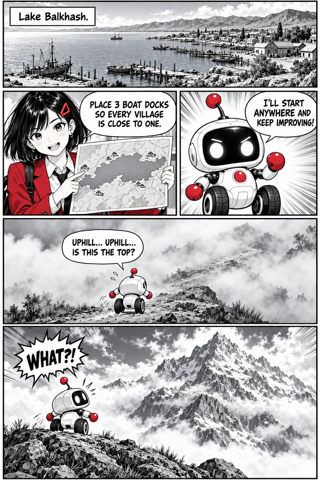
A* answers "which path?". Many problems instead ask "which configuration?": placing 8 queens with no attacks, ordering cities in a delivery tour (the Travelling Salesperson Problem, TSP), building a timetable, siting facilities. Local search keeps one (or a few) complete candidate solutions and tries to improve them by small changes. It uses very little memory: no big frontier, no explored set.
| Concept | Meaning | 8-queens example | TSP example |
|---|---|---|---|
| State | One complete configuration | 8 queens, one per column | A full tour A→C→B→D→A |
| Neighbour | A small change | Move one queen within its column | Swap two cities / reverse a segment (2-opt) |
| Objective function | One number: how good is it? | Number of attacking pairs (minimise) | Total tour length (minimise) |
Hill climbing
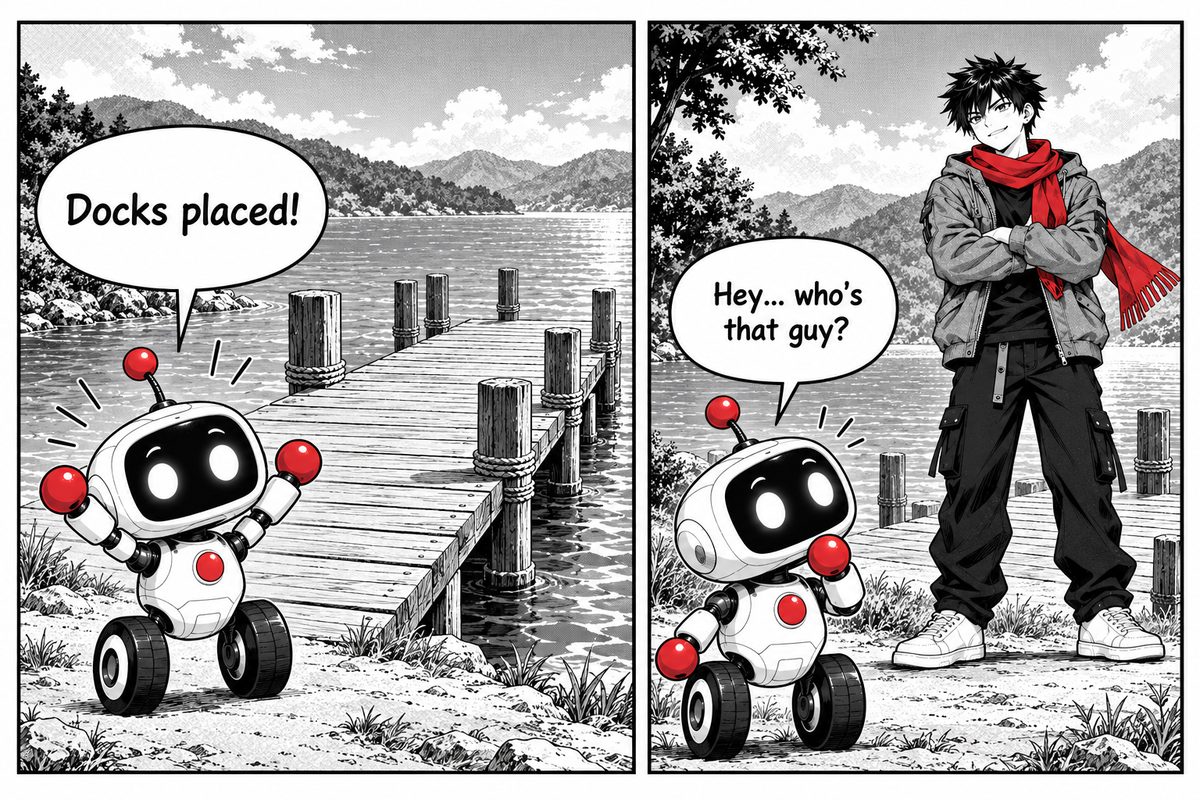
The simplest iterative improvement: move to the best neighbour while it is better than the current state; stop when no neighbour improves. It's like climbing a hill in thick fog by always stepping uphill.
def hill_climbing(values, start):
    current = start
    while True:
        neighbors = [i for i in (current-1, current+1) if 0 <= i < len(values)]
        best = max(neighbors, key=lambda i: values[i])
        if values[best] <= values[current]:
            return current               # no uphill move: a (local) peak
        current = best
Trace (lecture example): values = [1, 3, 5, 8, 6, 4, 2], start at index 0. Then 1 → 3 → 5 → 8. At 8 the neighbours are 5 and 6, neither better, so it returns index 3 (value 8).
Three ways hill climbing gets stuck
- Local maximum: higher than all neighbours, lower than another peak.
- Plateau: a flat area. No neighbour is better, so there's no direction to follow.
- Ridge: the good direction needs a sequence of moves that no single neighbour offers.
Escaping: restarts, annealing, beams, genes
Random-restart hill climbing runs hill climbing from several random starts and keeps the best result. It costs more computation but depends less on one unlucky start.
Simulated annealing sometimes accepts a worse move, with a probability controlled by a temperature T that slowly decreases (like cooling metal):
High T means the search explores and can cross valleys. Low T means it becomes greedy and refines. Cool too fast and it freezes in a poor spot; too slow and it wastes time. With slow enough cooling, theory guarantees convergence to the global optimum.
Local beam search keeps K states, generates all their successors, and keeps the best K overall. The K searches share information, so good regions attract the whole beam. Genetic algorithms keep a population, select by fitness, combine parents by crossover and add random mutation, generation after generation. In continuous spaces we can use gradient descent: step opposite the slope, x ← x − α∇f(x), where α is the step size (learning rate). This same idea trains the neural networks of Chapter 9.
Pick a method and press Run.
Start hill climbing at x = 8: it gets stuck on the first small peak. Random restarts usually find a higher peak. Annealing with a high start T often crosses valleys; with T = 1 it behaves almost like hill climbing. Annealing is random, so run it several times and compare.
Constraint Satisfaction Problems (CSP)
A CSP describes a problem by:
- Variables X₁…Xₙ (e.g. regions on a map),
- Domains: the allowed values for each variable ({red, green, blue}),
- Constraints: rules on combinations (two neighbouring regions must differ).
A solution assigns every variable a value with no constraint violated. Timetables, exam scheduling, Sudoku and map colouring are all CSPs. The textbook example colours the 7 regions of Australia with 3 colours.
Backtracking search assigns variables one at a time, checks constraints immediately, and backs up when a variable has no legal value left. Two simple tricks make it much faster:
- MRV (minimum remaining values): pick the variable with the fewest legal values left. "Fail first."
- Forward checking: after each assignment, remove now-illegal values from the neighbours' domains. If a domain becomes empty, backtrack at once.
Local search solves CSPs too. Min-conflicts starts with a full (possibly bad) assignment and repeatedly changes one conflicted variable to the value with the fewest conflicts. This works astonishingly well on n-queens, even with a million queens. The lecture's scheduling example turns constraints into a cost, Cost = 100T + 100R + 20S + 5W, and minimises it with local search.
Every region needs a colour that differs from all its neighbours. Conflicting edges turn red and dashed.
University timetabling, airline crew scheduling and delivery-route optimisation are solved with CSP and local-search tools such as Google OR-Tools, the same toolkit the lecture used for its TSP and scheduling examples.
Simulated annealing (Kirkpatrick, Gelatt & Vecchi, 1983) borrowed its maths from physics: slowly cooled metal settles into a low-energy crystal structure, while quenched metal stays brittle.
1. Why can hill climbing return a solution that is not the best?
2. In simulated annealing at high temperature, worse moves are…
3. In map colouring, what are the domains?